Constraints Anaysis

Download this as a Jupyter notebook

This example notebook illustrates xLA features that are useful for problems with constraints.

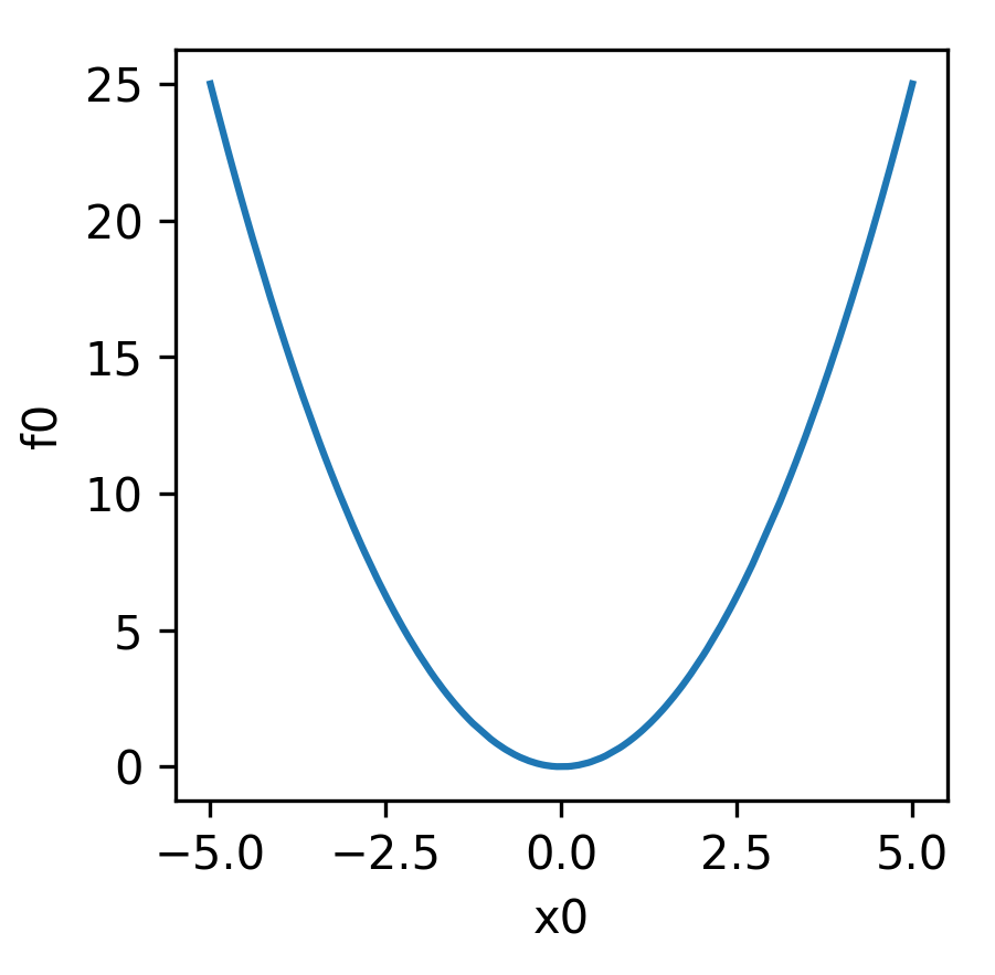
Lets defined a constrained sphere problem, with the sphere function as the objective:

(1)\[f_1(x) = x^2,\]

with the following constraints,

(2)\[v_0(x) = x^2 - 2 \leq 0,~\text{and}\]

(3)\[v_1(x) = 8 \cdot \sin(20 \cdot x) \leq 0.\]

The sphere function is visualised below:

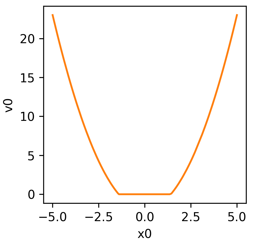
Equation (2) is visualised below:

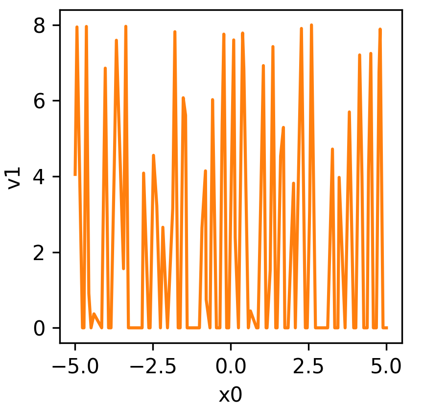
Equation (3) is visualised below:

Let us define the problem as a sample

from pyxla import load_data
from pyxla.sampling import HilbertCurveSampler
import math

sphere_f = lambda x: x** 2

sphere_sample = {
    "name": "Sphere",
    "X": HilbertCurveSampler(sample_size=100, dim=1, l_bound=-5, u_bound=5),
    "F": sphere_f,
    "V": [lambda x: sphere_f(x) - 2, lambda x: 8 * math.sin(20 * x)]
}

load_data(sphere_sample) # loaded in-place

WARNING:root:The Hilbert curve with dimension 1 is just a number line. You are sampling around points on a number line.

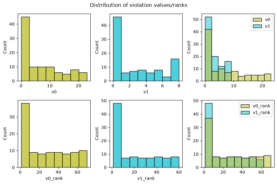
Violation distribution (distr_V)

pyxla.distr_v() can show the distribution of violation values for the two constraints:

from pyxla import distr_v

feat, plot = distr_v(sphere_sample)
feat

{'v0_min': 0.0,
 'v0_max': 23.0,
 'v0_mean': 6.696528453692529,
 'v0_med': 4.001720446035465,
 'v0_q1': 0.0,
 'v0_q3': 11.732460506067168,
 'v0_sd': 7.234727591773922,
 'v0_skew': 0.8207260120513635,
 'v0_kurt': -0.6125182736651693,
 'v0_feas_rate': 0.29,
 'v1_min': 0.0,
 'v1_max': 7.999601139849855,
 'v1_mean': 2.690866252454043,
 'v1_med': 0.0,
 'v1_q1': 0.0,
 'v1_q3': 6.1280500987167725,
 'v1_sd': 3.2206690112935923,
 'v1_skew': 0.5630104266641863,
 'v1_kurt': -1.431757575073753,
 'v1_feas_rate': 0.52,
 'overall_feas_rate': 0.16}

Pareto ranking distribution

from pyxla import distr_Par

distr_Par(sphere_sample)

({'paretoV_min': 0,
  'paretoV_max': 37,
  'paretoV_mean': 14.55,
  'paretoV_med': 13.0,
  'paretoV_q1': 5.0,
  'paretoV_q3': 23.75,
  'paretoV_sd': 11.457761693729847,
  'paretoV_skew': 0.3636548159197321,
  'paretoV_kurt': -1.0802420438914337,
  'paretoFV_min': 0,
  'paretoFV_max': 52,
  'paretoFV_mean': 26.2,
  'paretoFV_med': 27.0,
  'paretoFV_q1': 13.25,
  'paretoFV_q3': 38.75,
  'paretoFV_sd': 15.185718969020222,
  'paretoFV_skew': -0.051064472420160927,
  'paretoFV_kurt': -1.1570954601888022},
 <Figure size 600x300 with 2 Axes>)

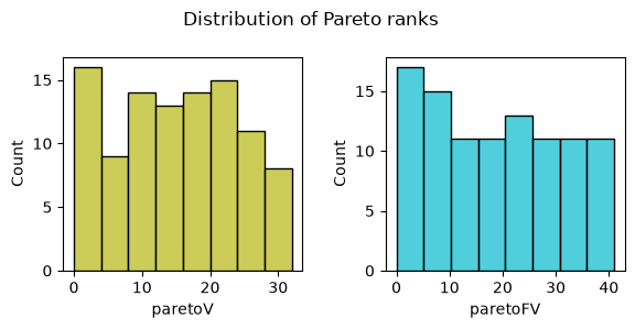
pyxla.distr_Par() gives an idea of how solutions rank against each other when the objective and the violation values are subjected to Pareto ranking.

Correlation among objective and violations and their ranks

from pyxla import corr, corr_ranks

corr, plot = corr(sphere_sample)
corr

/builds/aliefooghe/pyxla-wg/src/pyxla/__init__.py:376: ConstantInputWarning: An input array is constant; the correlation coefficient is not defined.
  cor, _ = spearmanr(x, y)

{'v0_f0 (feasible)': 'undefined',
 'v0_f0 (infeasible)': '1.00',
 'v1_f0 (feasible)': 'undefined',
 'v1_f0 (infeasible)': '-0.21',
 'v1_v0 (feasible)': 'undefined',
 'v1_v0 (infeasible)': '-0.22'}

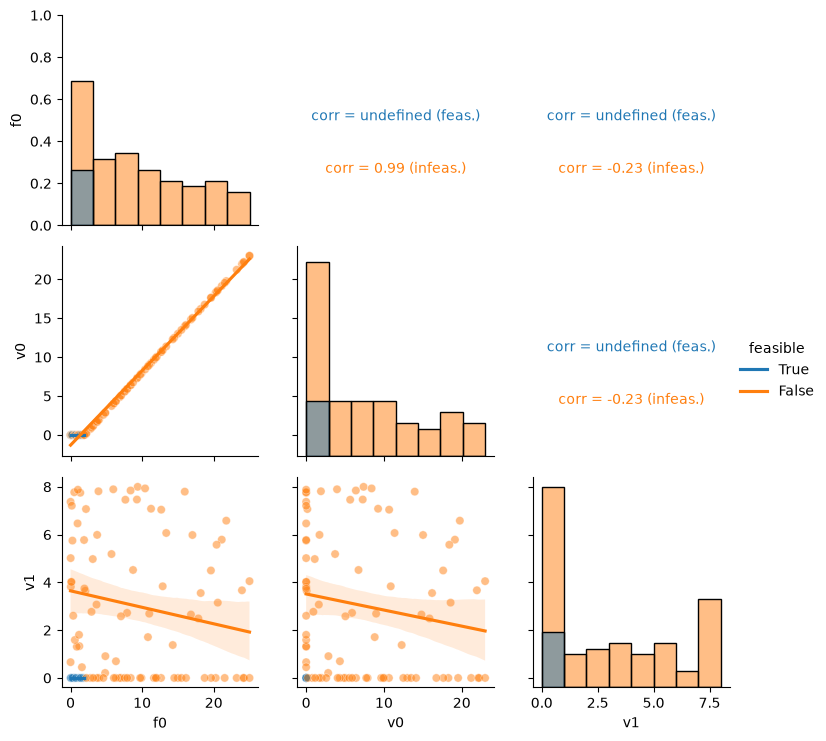
As expected the Equation (2) constraint is correlation with the objective (sphere function) and the Equation (3) constraint is not.

corr, plot = corr_ranks(sphere_sample)
corr

/builds/aliefooghe/pyxla-wg/src/pyxla/__init__.py:376: ConstantInputWarning: An input array is constant; the correlation coefficient is not defined.
  cor, _ = spearmanr(x, y)

{'v0_f0 (feasible)': 'undefined',
 'v0_f0 (infeasible)': '1.00',
 'v1_f0 (feasible)': 'undefined',
 'v1_f0 (infeasible)': '-0.21',
 'paretoV_f0 (feasible)': 'undefined',
 'paretoV_f0 (infeasible)': '0.95',
 'Deb_f0 (feasible)': '1.00',
 'Deb_f0 (infeasible)': '0.96',
 'paretoFV_f0 (feasible)': '1.00',
 'paretoFV_f0 (infeasible)': '1.00',
 'v1_v0 (feasible)': 'undefined',
 'v1_v0 (infeasible)': '-0.22',
 'paretoV_v0 (feasible)': 'undefined',
 'paretoV_v0 (infeasible)': '0.95',
 'Deb_v0 (feasible)': 'undefined',
 'Deb_v0 (infeasible)': '0.96',
 'paretoFV_v0 (feasible)': 'undefined',
 'paretoFV_v0 (infeasible)': '1.00',
 'paretoV_v1 (feasible)': 'undefined',
 'paretoV_v1 (infeasible)': '-0.03',
 'Deb_v1 (feasible)': 'undefined',
 'Deb_v1 (infeasible)': '-0.06',
 'paretoFV_v1 (feasible)': 'undefined',
 'paretoFV_v1 (infeasible)': '-0.18',
 'Deb_paretoV (feasible)': 'undefined',
 'Deb_paretoV (infeasible)': '1.00',
 'paretoFV_paretoV (feasible)': 'undefined',
 'paretoFV_paretoV (infeasible)': '0.96',
 'paretoFV_Deb (feasible)': '1.00',
 'paretoFV_Deb (infeasible)': '0.96'}

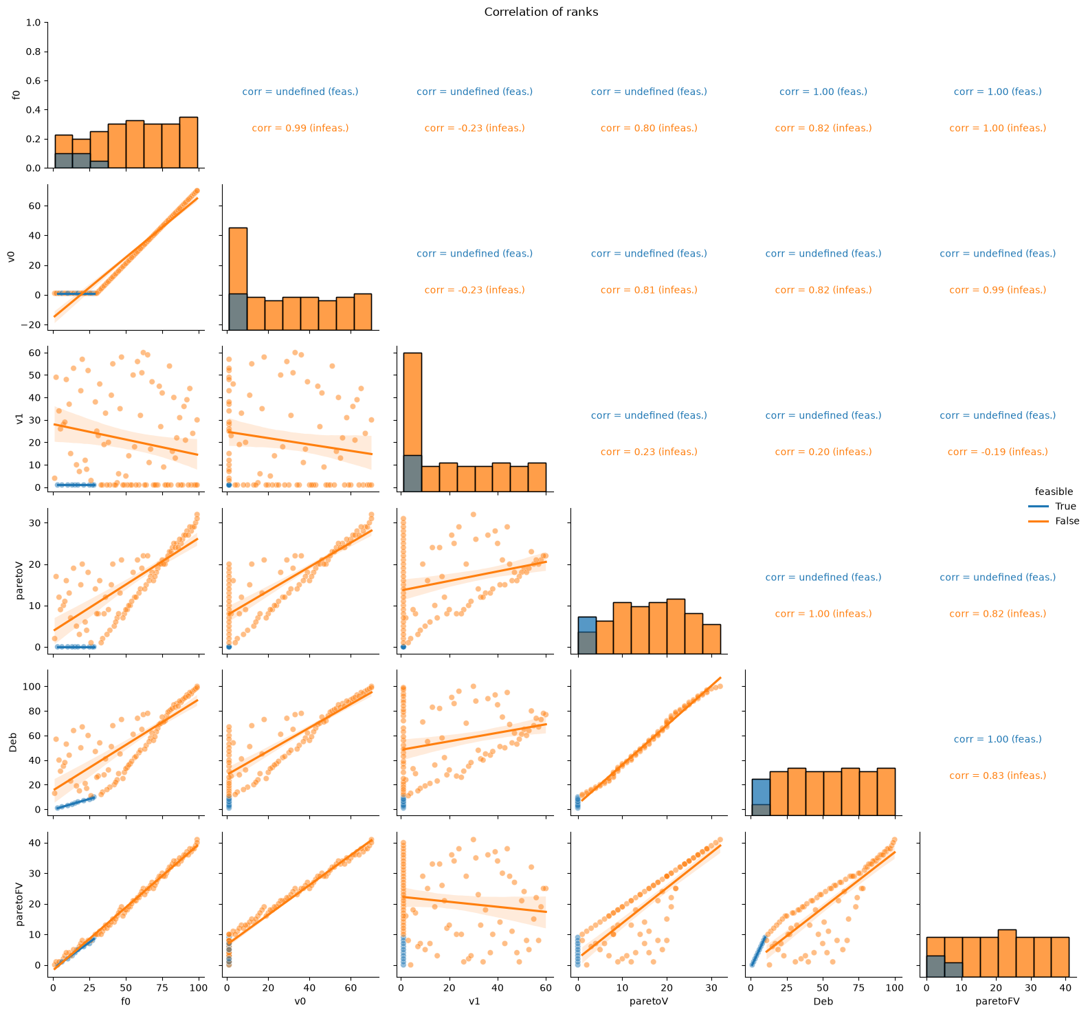
pyxla.corr_ranks() corroborates pyxla.corr() since it is based on the ranks rather than the values (objective or violation).

Violation distance correlation (VDC) and rank distance correlation (RDC)

from pyxla import vdc, rdc

corr, plot = vdc(sphere_sample)
corr

WARNING:root:No D file is present, thus, computing the D file... Computing an entire D file can be time consuming. Instead, you can call the function with the keyword argument `compute_D_file` set to `False` to speed up computation, as only the required distances will be calculated.

INFO:root:D file has been loaded to the current sample and is saved to ./Sphere_D.csv

{'vdc_v0': np.float64(0.9995891984690526),
 'vdc_v1': np.float64(-0.015848892748588795)}

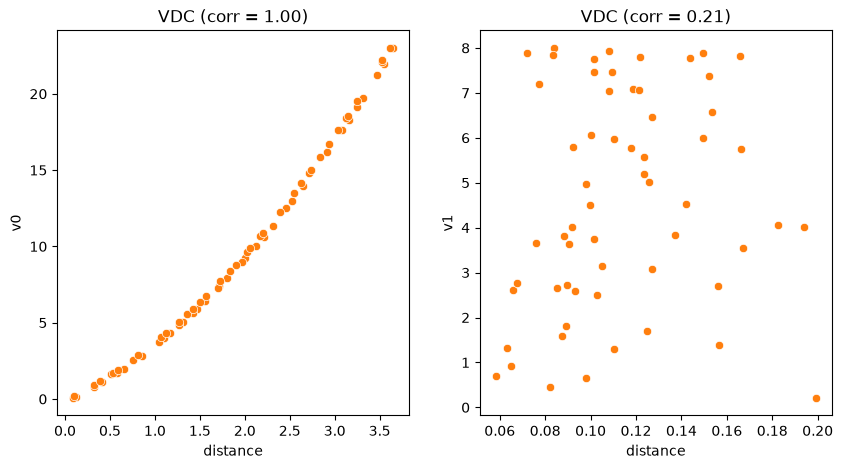
The violation values of the infeasible solutions of the Equation (2) constraint are highly correlated (0.9994) with the distance to the nearest feasible solutions. This implies that it is easy to cross to a feasible region from an infeasible region of solutions with respect to the Equation (2) constraint. Conversely, the low correlation coefficient of the Equation (3) constraint indicates a lower likelihood of crossing from an infeasible region to a feasible region.

corr, plot = rdc(sphere_sample)
corr

{'rdc_f0': np.float64(0.9967926696494598),
 'rdc_v0': np.float64(0.9998493137673016),
 'rdc_v1': np.float64(0.869323577054125),
 'rdc_paretoV': np.float64(0.7799345510669125),
 'rdc_Deb': np.float64(0.9472787278727871),
 'rdc_paretoFV': np.float64(0.9911171628546678)}

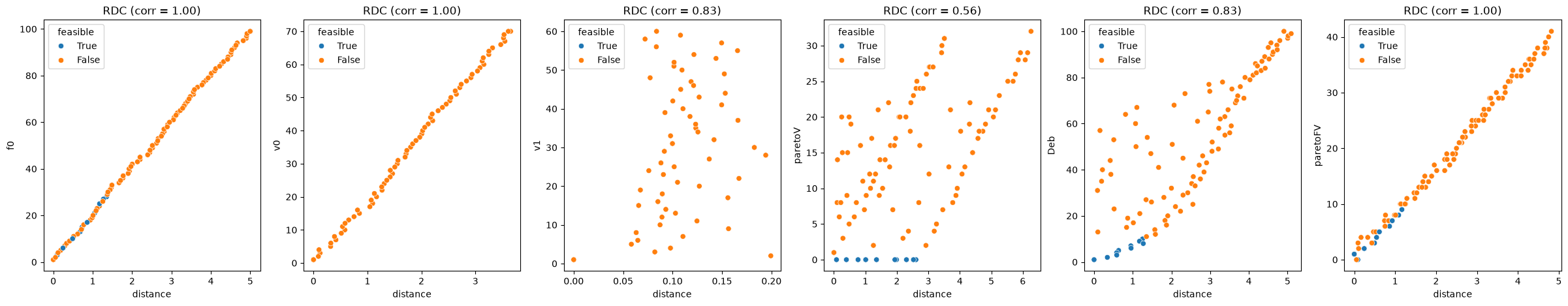
pyxla.rdc() corroborates pyxla.vdc() for the violation ranks.

Neighbouring solutions’ violation values correlation (NVC)

pyxla.nvc() indicates the level of searchability with respect to violation values.

from pyxla import nvc

corr, plot = nvc(sphere_sample)
corr

{'NVC_for_v0': 'nan', 'NVC_for_v1': 'nan'}

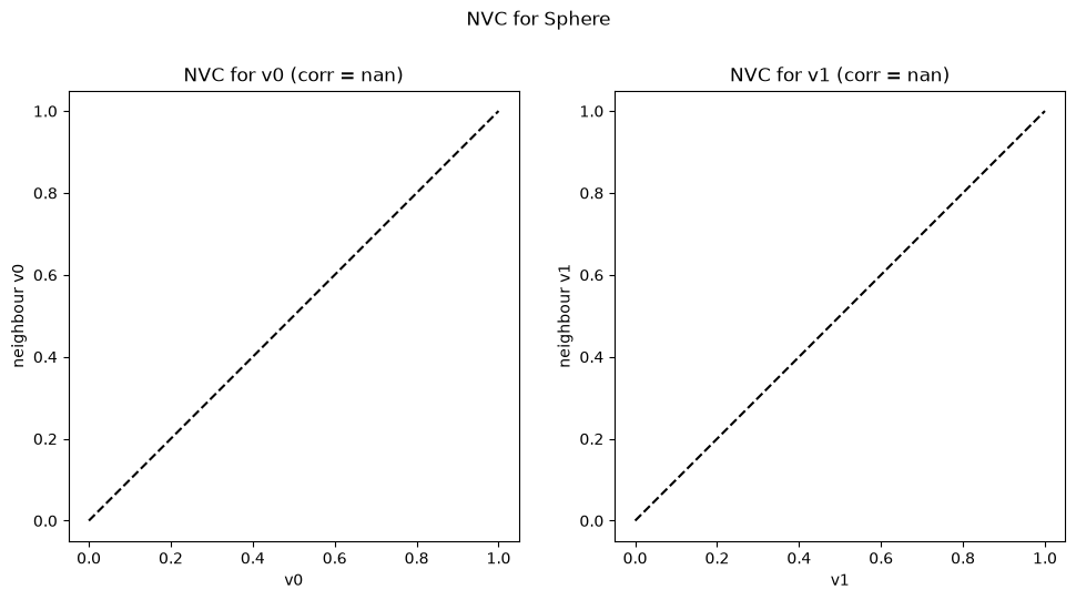
The Equation (2) constraint, being a simple sphere function, shows an almost perfect correlation. This indicates that there is high searchability with respect to the Equation (2) constraint: it is easy for a search to reach solutions of improving feasibility. Conversely, the Equation (3) constraint shows a weak negative correlation since, due to its cyclic nature, there is no strong relationship between violation values of neighbouring solutions. It is thus less likely for the search to continuously traverse along solutions of improving feasibility. Therefore, there is low searchability with respect to the Equation (3) constraint.