Comparing Continuous Problems
Download this as a Jupyter notebook
This example notebook shows how pyXla distinguishes between the sphere and deceptive problems.
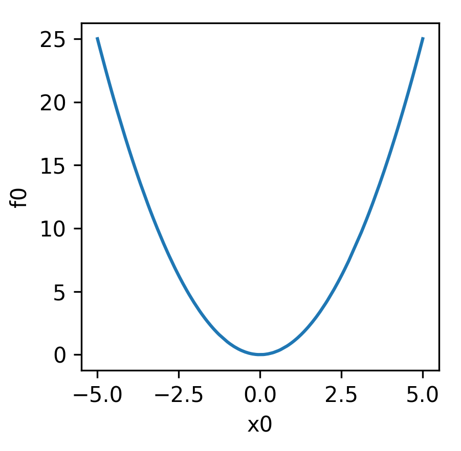
The sphere function is defined as:
and is visualised below:
The deceptive problem function is defined as:
and is visualised below:
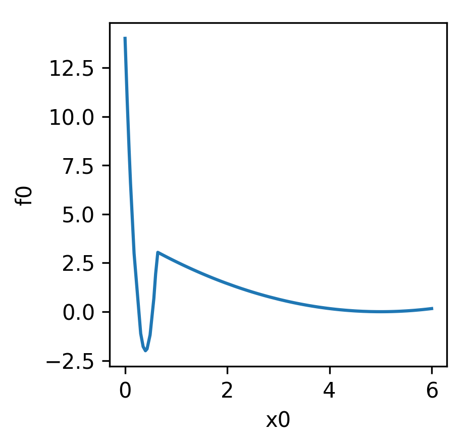
Equation (2) is called deceptive because it has two local minima as shown in its visualisation above.
To begin, we load the two problems as samples:
from pyxla import load_data
from pyxla.sampling import HilbertCurveSampler

sphere_sample = {
    "name": "Sphere",
    "X": HilbertCurveSampler(sample_size=100, dim=1, l_bound=-5, u_bound=5),
    "F": lambda x: x**2
}

deceptive_sample = {
    "name": "Deceptive",
    "X": HilbertCurveSampler(sample_size=100, dim=1, l_bound=0, u_bound=6),
    "F": lambda x: (0.4 * x - 2) ** 2 if x > 0.625 else (10 * x - 4) ** 2 - 2
}

load_data(sphere_sample) # loaded in-place
load_data(deceptive_sample) # loaded in-place
WARNING:root:The Hilbert curve with dimension 1 is just a number line. You are sampling around points on a number line.
WARNING:root:The Hilbert curve with dimension 1 is just a number line. You are sampling around points on a number line.
Compare their objective distribution:
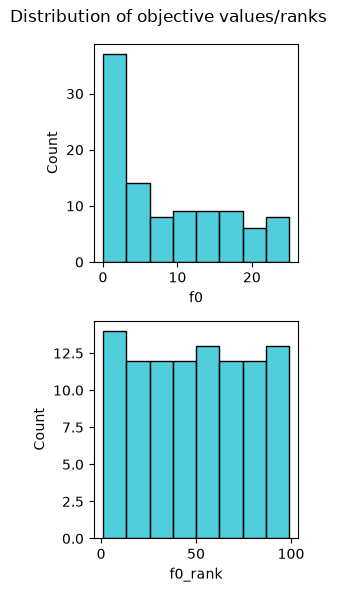
from pyxla import distr_f

feat, plot = distr_f(sphere_sample)
feat
{'f0_min': 0.0018248488999500836,
 'f0_max': 25.0,
 'f0_mean': 8.499871048531771,
 'f0_med': 6.122624575695372,
 'f0_q1': 1.3745772165871388,
 'f0_q3': 14.729325460917108,
 'f0_sd': 7.734905393983418,
 'f0_skew': 0.6024202344488225,
 'f0_kurt': -0.9579983133708163,
 'f0_rank_min': 1,
 'f0_rank_max': 99,
 'f0_rank_mean': 49.51,
 'f0_rank_med': 49.5,
 'f0_rank_q1': 24.25,
 'f0_rank_q3': 74.75,
 'f0_rank_sd': 28.99442475143569,
 'f0_rank_skew': 0.0019601813945263596,
 'f0_rank_kurt': -1.2027967085759266}
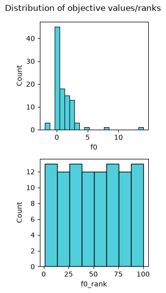
feat, plot = distr_f(deceptive_sample)
feat
{'f0_min': -1.9674534343370524,
 'f0_max': 14.0,
 'f0_mean': 1.0406091874802663,
 'f0_med': 0.5055989075010829,
 'f0_q1': 0.07254691205777361,
 'f0_q3': 1.688561507496938,
 'f0_sd': 1.8339746952884395,
 'f0_skew': 4.069748530322942,
 'f0_kurt': 24.608551370889696,
 'f0_rank_min': 1,
 'f0_rank_max': 100,
 'f0_rank_mean': 50.5,
 'f0_rank_med': 50.5,
 'f0_rank_q1': 25.25,
 'f0_rank_q3': 75.75,
 'f0_rank_sd': 29.011491975882016,
 'f0_rank_skew': 0.0,
 'f0_rank_kurt': -1.2002400240024003}
Fitness distance correlation (FDC) reveals more:
from pyxla import fdc

corr, plot = fdc(sphere_sample)
corr
WARNING:root:No D file is present, thus, computing the D file... Computing an entire D file can be time consuming. Instead, you can call the function with the keyword argument `compute_D_file` set to `False` to speed up computation, as only the required distances will be calculated.
INFO:root:D file has been loaded to the current sample and is saved to ./Sphere_D.csv
{'fdc_f0': np.float64(0.9994569440697371)}
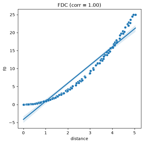
According to the output above, the sphere problem shows a high fitness-distance correlation between the objective values and distance to the nearest local minimum. This means that the search space is not deceptive, in that a search in the solution space will likely arrive at the global minimum since solutions become fitter and fitter as the search gets closer to the global minimum.
corr, plot = fdc(deceptive_sample)
corr
WARNING:root:No D file is present, thus, computing the D file... Computing an entire D file can be time consuming. Instead, you can call the function with the keyword argument `compute_D_file` set to `False` to speed up computation, as only the required distances will be calculated.
INFO:root:D file has been loaded to the current sample and is saved to ./Deceptive_D.csv
{'fdc_f0': np.float64(-0.7204680468046804)}
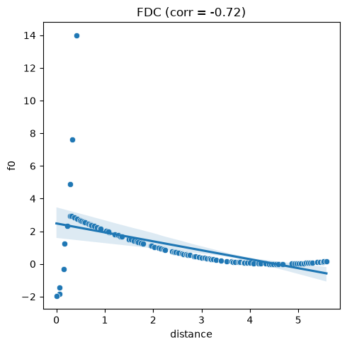
Conversely, the output above shows a negative correlation between distance to the nearest local minimum and objective values for the deceptive problem. Therefore, as one nears the global minimum, solutions tend to deteriorate in fitness, signalling the presence of multiple local minima. In this case, pyxla.fdc() indicates that the problem is indeed deceptive.
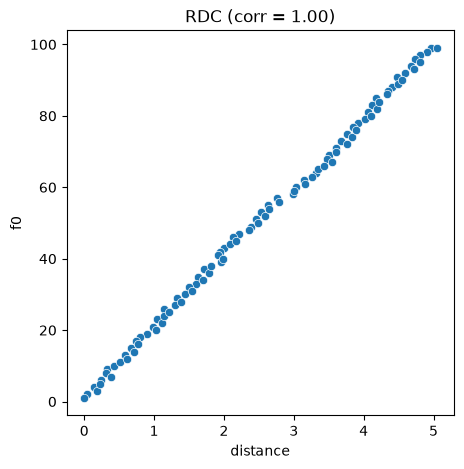
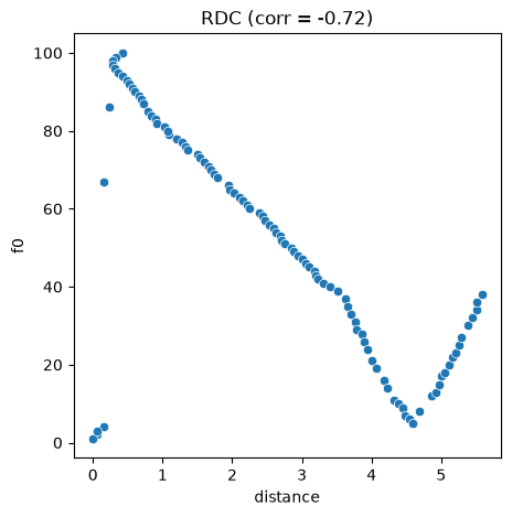
Rank distance correlation (RDC)
pyxla.rdc() corrobotates pyxla.fdc() since it operates on the objective ranks rather than the values.
from pyxla import rdc

corr, plot = rdc(sphere_sample)
corr
{'rdc_f0': np.float64(0.9994569440697371)}
corr, plot = rdc(deceptive_sample)
corr
{'rdc_f0': np.float64(-0.7204680468046804)}
Pairwise distance correlation (PDC)
from pyxla import pdc

corr, plot = pdc(sphere_sample)
corr
{'pdc_F': np.float64(0.4657671819056443),
 'pdc_f0-rank': np.float64(0.362336683172514)}
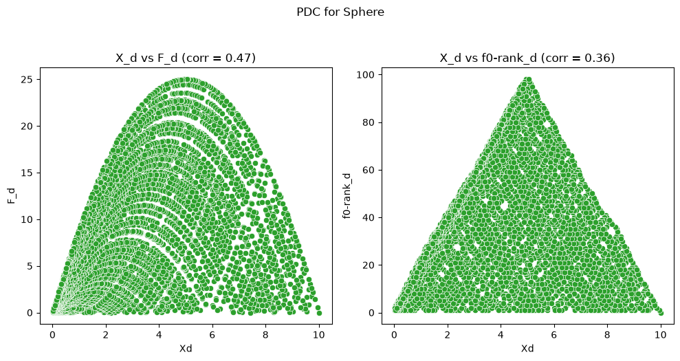
pyxla.pdc() shows that for the sphere function, there is low correlation between pairwise distance on the solution space and pairwise distance on the objective space. This shows that the sphere function is not monotonic.
corr, plot = pdc(deceptive_sample)
corr
{'pdc_F': np.float64(0.6741030730264398),
 'pdc_f0-rank': np.float64(0.7471429012937476)}
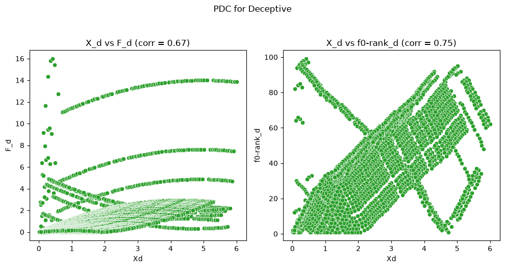
Similarly the deceptive function it not monotonic and appears more rugged that the sphere function.
Neighbouring solutions’ objective values (fitness) correlation (NFC)
from pyxla import nfc

corr, plot = nfc(sphere_sample)
corr
{'nfc_all_X_for_f0': np.float64(0.9970810142238714)}
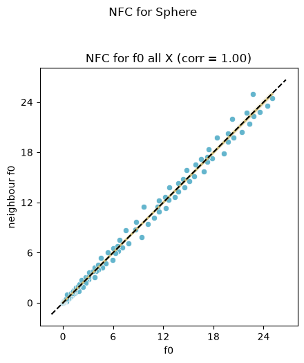
The constrained sphere problem is found to have high evolvability, evidenced by a high NFC value. This is expected, since the sphere function is one of the simplest continuous optimisation problems.
corr, plot = nfc(deceptive_sample)
corr
{'nfc_all_X_for_f0': np.float64(0.9263945578231292)}
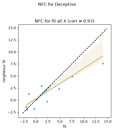
The deceptive problem has a high NFC but a lower value that the sphere function as expected, since the sphere problem is an easier problem.
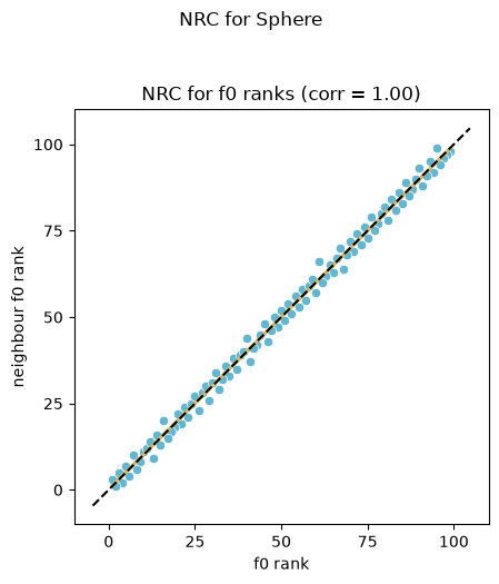
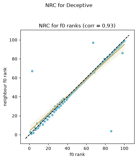
Neighbouring solutions’ ranks correlation (NRC)
pyxla.nrc() corroborates pyxla.nfc() since it is based on the objective ranks.
from pyxla import nrc

corr, plot = nrc(sphere_sample)
corr
{'NRC_for_f0_ranks': '0.9971'}
corr, plot = nrc(deceptive_sample)
corr
{'NRC_for_f0_ranks': '0.9264'}
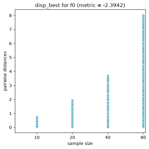
Dispersion of best solution (disp_best)
pyxla.disp_best() can tell if the problem has a global structure or whether it has many funnels.
from pyxla import disp_best

corr, plot = disp_best(sphere_sample)
corr
/builds/aliefooghe/pyxla/src/pyxla/__init__.py:1409: RuntimeWarning: divide by zero encountered in log
  forward = lambda x: np.log(x / init_percentage) / np.log(growth_factor)
{'f0': np.float64(-2.3942351222633955)}
corr, plot = disp_best(deceptive_sample)
corr
/builds/aliefooghe/pyxla/src/pyxla/__init__.py:1409: RuntimeWarning: divide by zero encountered in log
  forward = lambda x: np.log(x / init_percentage) / np.log(growth_factor)
{'f0': np.float64(0.7326295817082)}
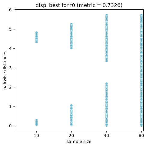
The sphere problem’s objective has a negative dispersion metric value which indicates the presence of a global structure, as expected. The deceptive problem, on the other hand, has a positive dispersion metric value, indicating the presence of funnels. The scatter plots visually express the dispersion, where for the constrained sphere problem, the spread of pairwise distances grows as the sample size of the best solution is increased. Conversely, for the deceptive problem, the gaps between the clusters of points for lower sample sizes show that indeed the best solutions are much further apart, accounting for the lack of a global structure.