pyxla¶

The core functions of the library. These function comprise xLA features.

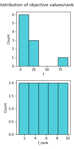
pyxla.distr_f(sample: dict, bins: int = 'auto') → Tuple[dict, Figure]¶

Computes the distribution of objectives (fitness values).

The distr_f feature visualises the spread of objective values and computes some descriptive statistics of the objective values. Alongside a histogram of objective values and a histogram of their dense ranking, various descriptive statistics are computed, including: minimum, maximum, mean, median, quartiles (Q1, Q3), standard deviation, skewness, and kurtosis. Dense ranking is a ranking method provided by the pandas package, which entails assigning to a group of equally valued solutions the least rank in the group and ensuring that rank increases by 1 from group to group.

Parameters:

sample (dict) – A sample containing the various input files i.e F, V.

Returns:

dict – Descriptive statistics of objective values.
matplotlib.figure.Figure – Histograms of objective values and or ranks of objective values.

Examples

>>> from pyxla import util, distr_f
>>> import matplotlib
>>> sample = util.load_sample('ackley8d_F1_V0', test=True)
>>> feat, plot = distr_f(sample)
>>> type(feat)
<class 'dict'>
>>> isinstance(plot, matplotlib.figure.Figure)
True

(Source code, png)

pyxla.distr_v(sample: dict) → Tuple[dict, Figure]¶

Computes the distribution of violation values.

The distr_v feature visualises the spread of violation values and computes some descriptive statistics of the violation values. Alongside a histogram of violation values and a histogram of their dense ranking, descriptive statistics are computed, including: minimum, maximum, mean, median, quartiles (Q1, Q3), standard deviation, skewness, and kurtosis. Additionally, the feasibility rate is computed per violation, and the overall feasibility, taking all constraints into account, is computed. Feasibility rate refers to the proportion of solutions that are feasible with respect to a constraint.

Parameters:

sample (dict) – A sample containing the various input files i.e F, V.

Returns:

dict – Descriptive statistics of violation values.
matplotlib.figure.Figure – Histograms of violation values and ranks of violation values.

Examples

>>> from pyxla import util, distr_v
>>> import matplotlib
>>> sample = util.load_sample('cec2010_c01_2d_F1_V2', test=True)
>>> feat, plot = distr_v(sample)
>>> type(feat)
<class 'dict'>
>>> isinstance(plot, matplotlib.figure.Figure)
True

(Source code, png)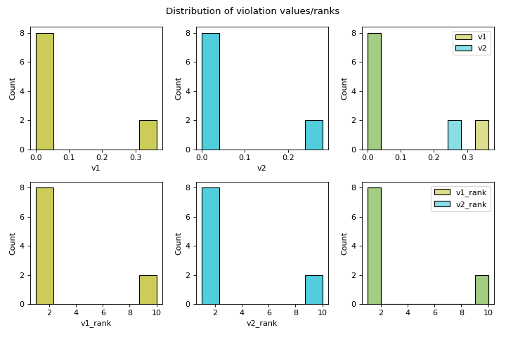

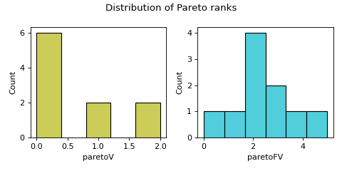
pyxla.distr_Par(sample: dict) → Tuple[dict, Figure]¶

Computes distribution of Pareto ranks.

The distr_Par feature produces a histogram of Pareto ranks and descriptive statistics on the ranks. This feature is applicable when there are at least two objectives or at least one constraint. Constraints are treated as objectives to be minimised in the Pareto ranking. The moocore package was used to compute Pareto rankings. Pareto ranking assigns ranks to solutions based on Pareto dominance. The solutions that are not dominated by any other solution are assigned rank 0. Ranking proceeds by excluding the first Pareto front and determining the next Pareto front, whose solutions will be given the next best rank. This proceeds till all the solutions have been ranked.

Parameters:

sample (dict) – A sample containing the various input files i.e F, V

Returns:

dict – Descriptive statistics of Pareto ranks
matplotlib.figure.Figure – Histogram(s) of Pareto ranks

Raises:

Exception – Raises an exception if a Pareto rank is not possible for the provided sample. The sample must have at least two objectives or at least one objective and constraint.

Examples

>>> from pyxla import util, distr_Par
>>> import matplotlib
>>> sample = util.load_sample('cec2010_c01_2d_F1_V2', test=True)
>>> feat, plot = distr_Par(sample)
>>> type(feat)
<class 'dict'>
>>> isinstance(plot, matplotlib.figure.Figure)
True

(Source code, png)

pyxla.distr_Deb(sample: dict) → Tuple[dict, FacetGrid]¶

Computes Deb’s Feasibility Rule Ranking Distribution.

Solutions were ranked following Deb’s feasibility rule ranking where solutions are ranked based on three criteria: (1) feasible solutions are ranked as better than infeasible solutions, (2) among two feasible solutions, the one with a better objective value is ranked better, and (3) among infeasible solutions, solutions with lower violation values are ranked better [1]. This was implemented by summing up scaled objective ranks with violation ranks and ranking solutions based on the result of summation using dense ranking. The objective ranks are scaled to the range [0, 1] by dividing each rank by the maximum rank plus 1, resulting in a real value below 1. Thus, for each solution, the violation ranks with respect to each violation and the scaled objective rank are summed. Additionally, descriptive statistics for the computed ranks are calculated.

Parameters:

sample (dict) – A sample containing the various input files i.e F, V

Returns:

dict – Descriptive statistics of Pareto ranks
sns.axisgrid.FacetGrid – Histogram of Deb’s feasibility rule ranks

Examples

>>> from pyxla import util, distr_Deb
>>> import seaborn
>>> sample = util.load_sample('cec2010_c01_2d_F1_V2', test=True)
>>> feat, plot = distr_Deb(sample)
>>> type(feat)
<class 'dict'>
>>> isinstance(plot, seaborn.axisgrid.FacetGrid)
True

(Source code, png)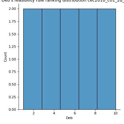

pyxla.corr(sample: dict) → Tuple[dict, PairGrid]¶

Computes correlation of values.

This feature creates a scatter plot for all pair combinations of objectives and violations. For each pair, the Spearman’s correlation coefficient is calculated. Concretely, for a problem with one objective and two constraints, this feature creates a scatter plot of the objective values against violation values of the first constraint, another scatter plot of objective values against violation values of the second constraint, and finally a scatter plot of violation values of the first constraint against those of the second constraint. For each of these scatter plots the Spearman’s correlation is calculated as numerical output. Further, the scatter plots and correlation calculations are split by feasibility. Correlations involving feasible solutions are undefined, as all violation values are zero.

Parameters:

sample (dict) – A sample containing the various input files i.e F, V.

Returns:

dict – Spearman’s correlation coefficients for all pairs of sets of values split by feasibility
sns.PairGrid – Grid of scatter plots of all objectives and violations against each other, with feasibility indicated per solution.

Examples

>>> from pyxla import util, corr
>>> import seaborn
>>> sample = util.load_sample('cec2010_c01_2d_F1_V2', test=True)
>>> feat, plot = corr(sample)
>>> type(feat)
<class 'dict'>
>>> isinstance(plot, seaborn.PairGrid)
True

(Source code, png)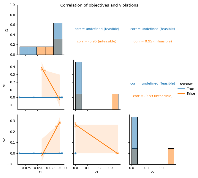

pyxla.corr_ranks(sample: dict) → Tuple[dict, PairGrid]¶

Computes correlation of ranks.

This feature creates scatter plots and calculates Spearman’s correlation values for all pairs of ranks objectives and violations, Pareto ranks, and Deb’s ranks. For instance, violation ranks can be plotted against objective ranks. Similarly, the scatter plots and correlation calculations are split by feasibility. Correlation involving feasible solutions may be undefined since these solutions tend to have the same violation value ranks and Pareto ranks involving constraints, hence such sets have zero standard deviation. Consequently, for feasible solutions, Spearman’s correlation coefficient is undefined.

Parameters:

sample (dict) – A sample containing the various input files i.e F, V

Returns:

sns.PairGrid – Grid of scatter plots of all objective, violation, Pareto and Deb’s ranks against each other, with feasibility indicated per solution
dict – Spearman’s correlation coefficients for all pairs of sets of ranks split by feasibility

Examples

>>> from pyxla import util, corr_ranks
>>> import seaborn
>>> sample = util.load_sample('cec2010_c01_2d_F1_V2', test=True)
>>> feat, plot = corr_ranks(sample)
>>> type(feat)
<class 'dict'>
>>> isinstance(plot, seaborn.PairGrid)
True

(Source code, png)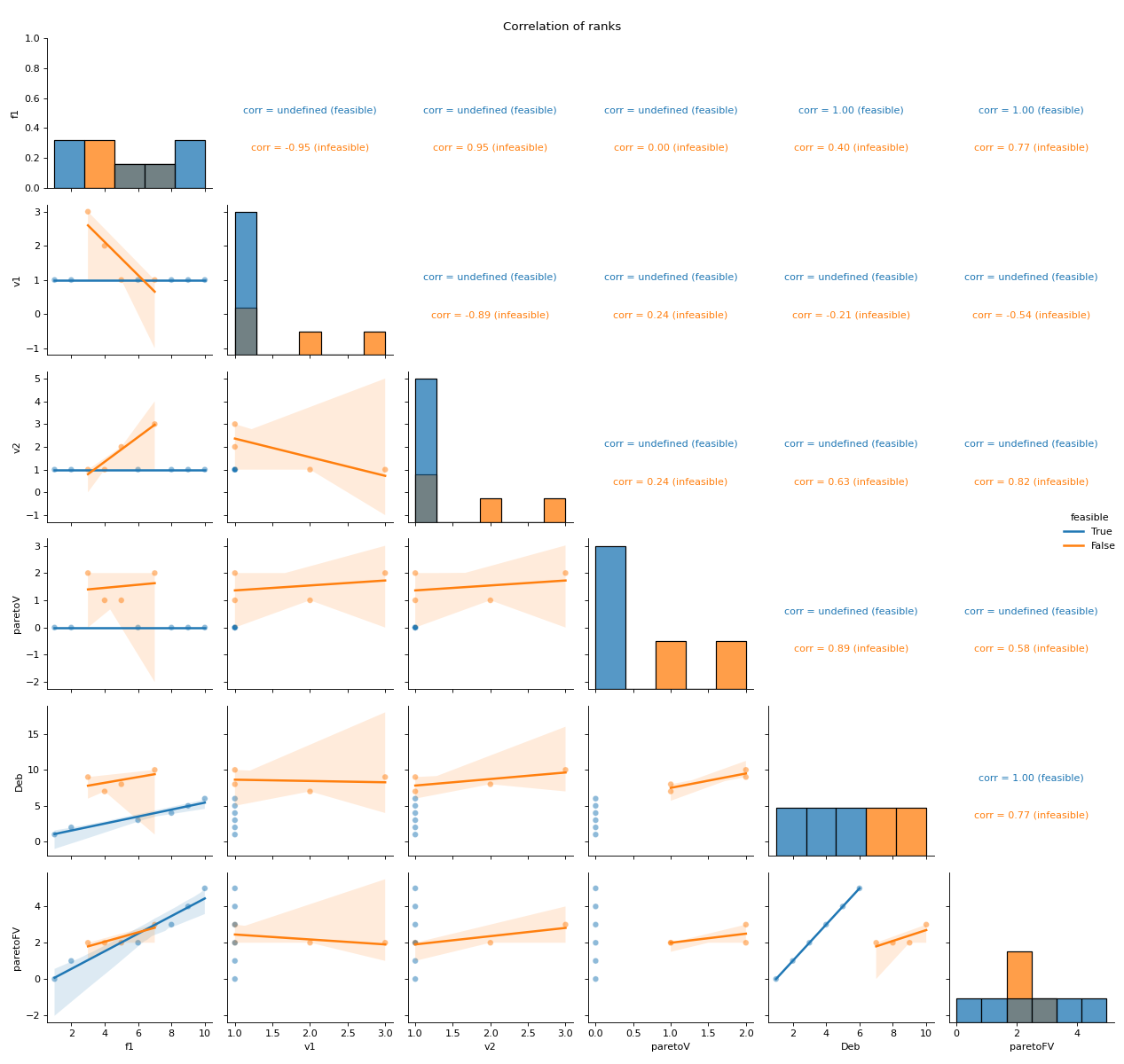

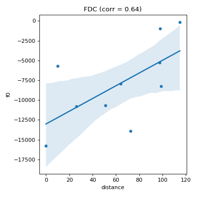
pyxla.fdc(sample: dict, compute_D_file: bool = True) → Tuple[dict, Figure]¶

Computes objective (fitness) distance correlation (FDC).

This feature is an implementation of the method proposed by Jones and Forrest [3]. For each set of objective values \(F_i\), a pair \((f_i, d_i)\) is generated for each solution, where \(f_i\) is the fitness of solution \(i\), and \(d_i \in D_i\) is the distance between solution \(i\) and the nearest best solution. This feature produces, as visual output, a scatter plot of fitness (\(F_i\)) against distance (\(D_i\)) and calculates Spearman’s correlation coefficient between \(F_i\) and \(D_i\) as the corresponding numerical output for each objective for feasible and infeasible solutions separately.

Parameters:

sample (dict) – A sample containing the various input files i.e `F`, `V`.
compute_D_file (bool, optional) – By default `True`; when there is no D file in the sample, if `compute_D_file` is set to `True`, the whole D file is calculated. Calculating the whole D file will eliminate redundant distance calculations in the future, but it can be time consuming. To speed up calculation of fdc, set `compute_D_file` to `False` so that only the required distances are calculated.

Returns:

dict – Dictionary containing Spearman’s correlation coefficients objective-distance correlation per objective.
matplotlib.figure.Figure – matplotlib axes containing scatter plots of objective values against distance to the nearest best solution in sample per objective, for all solutions or for feasible solutions only.

Raises:

Exception – Raises an exception if both D and X inputs are absent. One of D or X is needed to compute distances between solution.

Examples

>>> from pyxla import util, fdc
>>> import matplotlib
>>> sample = util.load_sample('sphere', test=True)
>>> feat, plot = fdc(sample)
>>> type(feat)
<class 'dict'>
>>> isinstance(plot, matplotlib.figure.Figure)
True

(Source code, png)

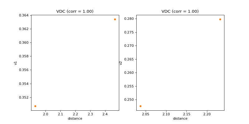
pyxla.vdc(sample: dict, compute_D_file: bool = True) → Tuple[dict, Figure]¶

Calculates violation distance correlation (VDC).

This feature was implemented by extending the objective-distance correlation feature (pyxla.fdc()) to violation values. For each set of violation values \(V_i\) and for infeasible solutions only, a pair \((v_i, d_i)\) is generated where \(v_i\) is the violation value of solution \(i\), and \(d_i \in D_i\) is the distance between solution \(i\) and the nearest feasible solution. This feature produces, as visual output, a scatter plot of violation (\(V_i\)) against distance (\(D_i\)) and calculates Spearman’s correlation coefficient between \(V_i\) and \(D_i\) as the corresponding numerical output for each constraint. This feature is only applicable to constrained problems. The feature is applied to infeasible solutions only because all feasible solutions have a violation value of zero.

Parameters:

sample (dict) – A sample containing the at least input files V and D.
compute_D_file (bool, optional) – By default True; when there is no D file in the sample, if compute_D_file is set to True, the whole D file is calculated. Calculating the whole D file will eliminate redundant distance calculations in the future, but it can be time consuming. To speed up calculation of fdc, set compute_D_file to False so that only the required distances are calculated.

Returns:

dict – Dictionary containing correlation between constraints and distance to the nearest feasible solution.
matplotlib.figure.Figure – `matplotlib` axes containing a scatter plot of violation values against distance to the nearest feasible solution.

Examples

>>> from pyxla import util, vdc
>>> import matplotlib
>>> sample = util.load_sample('cec2010_c01_2d_F1_V2', test=True)
>>> corr, plot = vdc(sample)
>>> type(corr)
<class 'dict'>
>>> isinstance(plot, matplotlib.figure.Figure)
True

(Source code, png)

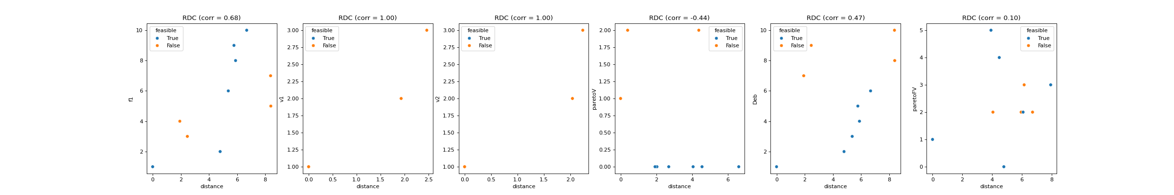
pyxla.rdc(sample: dict, compute_D_file: bool = True) → Tuple[dict, Figure]¶

Computes rank distance correlation (RDC).

This feature was implemented by extending the objective-distance correlation feature (pyxla.fdc()) to ranks. For each rank \(R_i\), a pair \((r_i, d_i)\) is generated for each solution, where \(r_i\) is the rank of solution \(i\), and \(d_i \in D_i\) is the distance between solution \(i\) and the nearest best solution. The visual output is a scatter plot of ranks (\(R_i\)) against distances (\(D_i\)), and calculates Spearman’s correlation coefficient between \(R_i\) and \(D_i\) as the corresponding numerical output for each rank.

Parameters:

sample (dict) – A sample containing the at least input files V and D.
compute_D_file (bool, optional) – By default True; when there is no D file in the sample, if compute_D_file is set to True, the whole D file is calculated. Calculating the whole D file will eliminate redundant distance calculations in the future, but it can be time consuming. To speed up calculation of fdc, set compute_D_file to False so that only the required distances are calculated.

Returns:

dict – Dictionary containing correlation between ranks and distance to the nearest best solution.
matplotlib.figure.Figure – matplotlib axes containing a scatter plot of ranks against distance to the nearest best solution.

Examples

>>> from pyxla import util, rdc
>>> import matplotlib
>>> sample = util.load_sample('cec2010_c01_2d_F1_V2', test=True)
>>> feat, plot = rdc(sample)
>>> type(feat)
<class 'dict'>
>>> isinstance(plot, matplotlib.figure.Figure)
True

(Source code, png)

pyxla.pdc(sample: dict, metric: Callable | str = 'euclidean') → Tuple[dict, Figure]¶

Computes pairwise distance correlation (PDC).

This feature is based on Mantel’s standardised test [2], which was applied in population genetics to determine whether and to what extent geographic distance influences genetic distance. The PDC| feature applies Mantel’s standardised test to analyse the relationship between pairwise distance on the solution space and pairwise distance on the objective space (all objectives), violation space (all violations), and for each objective, violation, and rank independently. The scipy package was used to efficiently compute pairwise distances. The feature produces scatter plots of pairwise distance on the solution space against pairwise distance on the objective space (all objectives), violation space (all violations), and against each objective, violation, and rank. The corresponding numerical outputs are the Spearman’s correlation coefficients between each set of pairwise distances.

Parameters:

sample (dict) – A sample containing the at least input files V and D.
metric (Callable or str, optional) – A metric function or the name of a distance metric as listed scipy’s pdist function. If a metric function is defined it must take two solutions and computes distance between them of the form dist(Xa, Xb) -> d where Xa and Xb are pandas Series representing solutions, by default None. For example: lambda Xa, Xb: abs(Xa.sum() - Xb.sum()).

Returns:

dict – Dictionary containing correlation between pairwise distance on the solution space and pairwise distance on the objective space, on the violation space, and on each objective, violation and rank individually.
matplotlib.figure.Figure – matplotlib axes containing a scatter plot of pairwise distance on the solution space against pairwise distance on the objective space, on the violation space, and on each objective, violation and rank individually.

Examples

>>> from pyxla import util, pdc
>>> import matplotlib
>>> sample = util.load_sample('cec2010_c01_2d_F1_V2', test=True)
>>> corr, plot = pdc(sample)
>>> type(corr)
<class 'dict'>
>>> isinstance(plot, matplotlib.figure.Figure)
True

(Source code, png)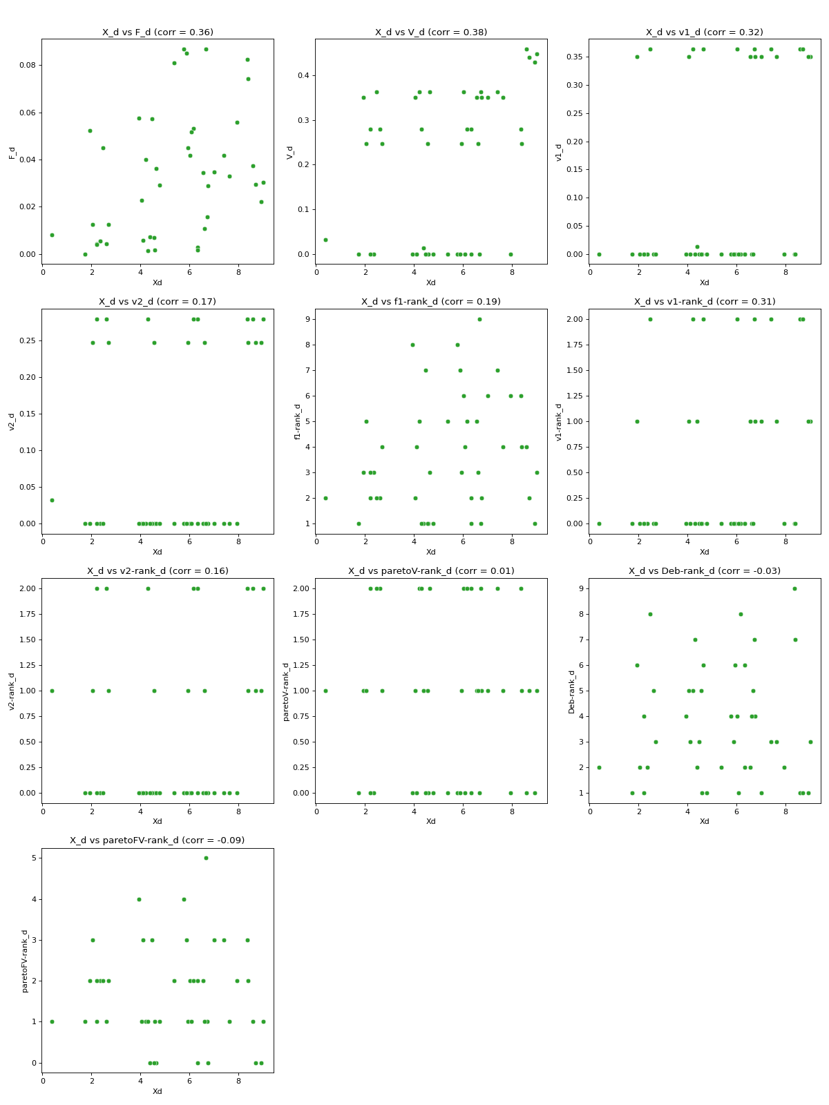

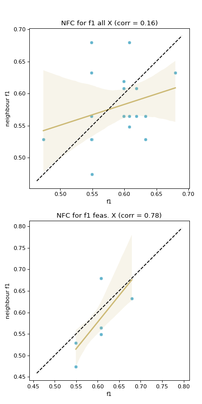
pyxla.nfc(sample: dict) → Tuple[dict, Figure]¶

Computes neighbouring solutions’ objective values (fitness) correlation (NFC).

This feature is implemented following the fitness cloud technique proposed by Verel et al. [6]. Verel et al. proposed the technique to analyse the correlation between objective values of parents and offspring in the context of evolutionary computing.

The fitness cloud technique was applied to analyse the correlation of fitness values between pairs of neighbours in a sample. Therefore, a neighbourhood file N is required. Considering each objective, for all pairs of neighbours, the corresponding objective values for each pair are plotted against each other in a scatter plot to produce a fitness cloud [5]. A regression line is overlaid on the scatter plot. Further, a dotted identity line is plotted such that, assuming minimisation, points above it indicate deteriorating neighbours, those below it are improving neighbours, and those on the line are neutral neighbours. This procedure is done considering all solutions, and then considering feasible solutions only. The result is a pair of scatter plots for each objective. The numerical output of NFC is the Spearman’s correlation coefficient between fitness values of solutions on the \(x\)-axis and those on the \(y\)-axis. Similarly, correlation is calculated considering all solutions and for feasible solutions only. NFC highlights the level of evolvability of fitness of a search space. Evolvability of a search space can be defined as the level of likelihood that a search reaches an area of better fitness in a landscape.

Parameters:

sample (dict) – A sample containing input files i.e F, N.

Returns:

dict – Dictionary containing correlation between objective values of solutions and the objective values of their neighbours, for all solutions and for feasible solutions only.
matplotlib.axes.Axes – matplotlib axes each containing a scatter plot of objective values of solutions against the objective values of their neighbours, for all solutions and for feasible solutions only.

Raises:

Exception – Raised if both N and X inputs are absent, as neighbourhood cannot be determined without having either.

Examples

>>> from pyxla import util, nfc
>>> import matplotlib
>>> sample = util.load_sample('nk_n14_k2_id5_F1_V1', test=True)
>>> corrs, plot = nfc(sample)
>>> type(corrs)
<class 'dict'>
>>> isinstance(plot, matplotlib.figure.Figure)
True

(Source code, png)

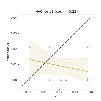
pyxla.nvc(sample: dict) → Tuple[dict, Figure]¶

Computes neighbouring solutions’ violation values correlation (NVC)

This feature was implemented by extending the fitness cloud technique of pyxla.nfc() to the violation values. Considering infeasible solutions only with respect to each constraint, for all pairs of neighbours, the corresponding violation values are plotted against each other in a scatter plot. Similarly, a regression line is overlaid on the scatter plot. Further, a dotted identity line is plotted such that points above it indicate deteriorating neighbours, those below it are improving neighbours, and those on the line are neutral neighbours. The result is a scatter plot for each constraint. The corresponding numerical output for each plot is Spearman’s correlation coefficient between violation values on the \(x\)-axis and those on the \(y\)-axis. Only infeasible solutions are considered, because feasible solutions have a violation value of zero. NVC indicates the level of searchability with respect to violation values; it quantifies how likely it is for a search to reach an area of the search space of lower constraint violation.

Parameters:

sample (dict) – A sample containing input files i.e V, N.

Returns:

dict – Dictionary containing correlation between violation values of solutions and the violation values of their neighbours, for infeasible solutions only.
matplotlib.axes.Axes – matplotlib axes each containing a scatter plot of violation values of solutions against the violation values of their neighbours for infeasible solutions only.

Examples

>>> from pyxla import util, nvc
>>> import matplotlib
>>> sample = util.load_sample('nk_n14_k2_id5_F3_V2', test=True)
>>> corrs, plot = nvc(sample)
>>> type(corrs)
<class 'dict'>
>>> isinstance(plot, matplotlib.figure.Figure)
True

(Source code, png)

pyxla.nrc(sample: dict) → Tuple[dict, Figure]¶

Computes neighbouring solutions’ ranks correlation (NRC).

This feature was implemented by extending the fitness cloud technique of pyxla.nfc() to ranks, such that fitness values are substituted with ranks. Considering each rank, for all pairs of neighbours, the corresponding ranks are plotted against each other in a scatter plot. A regression line is overlaid on the scatter plot. Further, a dotted identity line is plotted such that points above it indicate improving neighbours, those below it are deteriorating neighbours, and those on the line are neutral neighbours. The result is a scatter plot for each rank. The corresponding numerical output for each plot is Spearman’s correlation coefficient between rank values on the \(x\)-axis and those on the \(y\)-axis. Similarly, NRC indicates searchability with regard to the various ranks.

Parameters:

sample (dict) – A sample containing input files i.e F, N.

Returns:

dict – Dictionary containing correlation between ranks of solutions and the ranks of their neighbours.
matplotlib.axes.Axes – matplotlib axes each containing a scatter plot of ranks of solutions against the ranks of their neighbours.

Examples

>>> from pyxla import util, nrc
>>> import matplotlib
>>> sample = util.load_sample('nk_n14_k2_id5_F3_V2', test=True)
>>> corrs, plot = nrc(sample)
>>> type(corrs)
<class 'dict'>
>>> isinstance(plot, matplotlib.figure.Figure)
True

(Source code, png)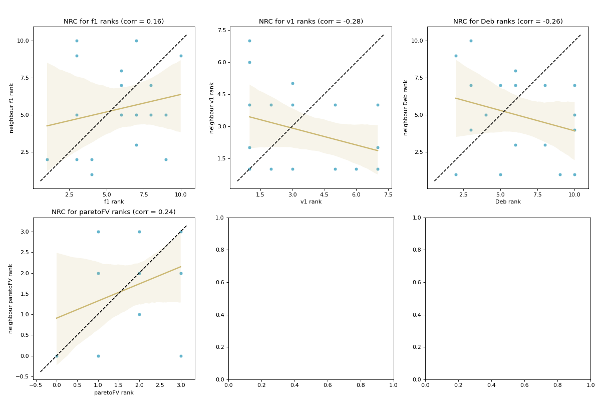

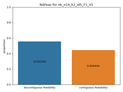
pyxla.ncf(sample: dict) → Tuple[dict, Axes]¶

Computes neighbouring change in feasibility (NΔFeas).

The NΔFeas feature was implemented as an algorithm that uses a neighbourhood file, N, to compute the proportion of transitions from one solution to another that result in a change in feasibility and the proportion of transitions that do not result in a change in feasibility. The numerical output produced is a set of proportions, while the visual output is a bar chart of the proportions. This feature shows the extent to which regions of infeasible or feasible solutions are contiguous. The level of contiguousness is indicative of the evolvability of the landscape with regard to feasibility.

Parameters:

sample (dict) – A sample containing input files i.e F, N.

Returns:

proportions (dict) – Dictionary containing the numerical proportions as defined above.
matplotlib.axes.Axes – matplotlib figure with the bar chart visually illustrating the proportions defined above.

Raises:

Exception – Raises an exception if no V file is provided as feasibility is undefined without the V file.
Exception – Raises an exception if the sample only has solutions belong to only one class of feasibility i.e if all solutions are infeasible or if all solutions are feasible.
Exception – Raised if both N and X inputs are absent, as neighbourhood cannot be determined without having either.

Examples

>>> from pyxla import util, ncf
>>> sample = util.load_sample('nk_n14_k2_id5_F1_V1', test=True)
>>> proportions, fig = ncf(sample)
>>> proportions

(Source code, png)

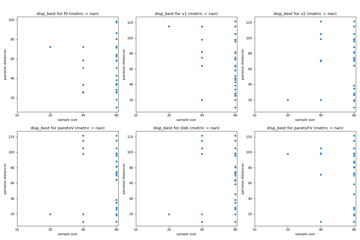
pyxla.disp_best(sample: dict, init_percentage: int = 10, growth_factor: int = 2) → Tuple[dict, Figure]¶

Computes dispersion of best solutions (disp_best).

The implementation of the disp_best feature is based on the dispersion metric proposed by Lunacek and Whitley [4]. Initially, the overall sample of solutions is sorted according to some rank. Subsamples of the \(n\) best solutions are obtained from that sample where \(n\) increases according to a specified geometric growth factor. For each subsample, the pairwise distance among the contained solutions is calculated. The visual output of disp_best is a scatter plot of sample size against pairwise distances. The corresponding numerical output is the dispersion metric computed by subtracting the average of pairwise distances (dispersion) of the largest subsample from the average of pairwise distances of the smallest subsample. Lower dispersion metric values indicate the presence of a global structure, while higher values indicate the presence of funnels. Thus, disp_best indicates the presence (and the extent thereof) or the absence of multimodality.

Parameters:

sample (dict) – A sample containing input files i.e F, N.
init_percentage (int, optional) – Intial subsample size in percentage, by default 10
growth_factor (int, optional) – Defines how to successively increase sample size, by default 2

Returns:

dict – Dictionary containing dispersion metrics for each subsample size.
matplotlib.figure.Figure – matplotlib scatter plots of subsample size against pairwise distances.

Raises:

Exception – Raised if initial percentage size of a subsample is \(\geq100%\).

Examples

>>> from pyxla import util, disp_best
>>> import matplotlib
>>> sample = util.load_sample('sphere', test=True)
>>> feat, plot = disp_best(sample)
>>> type(feat)
<class 'dict'>
>>> isinstance(plot, matplotlib.figure.Figure)
True

(Source code, png)

pyxla.X_imp(sample: dict, binary: bool = False, n_repeats: int = 10, train_proportion: int = 0.7, estimator: Literal['ridge', 'lasso', 'lars'] = 'lasso', alpha: float = 1, seed: float = None) → Tuple[DataFrame, dict, Figure]¶

Computes variable importance (X_imp)

The implementation of the X_imp feature produces a bar chart of correlation values between each decision variable in the X file and each objective in the F file. Correlation is calculated as Spearman’s correlation coefficient except for problems where a decision variable is binary, in which case the point-biserial correlation coefficient is calculated instead. Additionally, a linear regression model is fitted on X as features and F as the output. The scikit-learn is utilised for this. The feature allows the desired regression model to be specified as a parameter, i.e., Ridge or Lasso. The features are scaled to values between 0 and 1 to ensure all features contribute equally. The linear model is used to carry out permutation variable importance using a function provided by the scikit-learn package. Each variable is permuted to random values, and the effect on the predicted objective value is quantified over a number of repetitions.

Parameters:

sample (dict) – A sample containing input files i.e F, X.
binary (bool, optional) – Set to True if the sample involves variables from a discrete domain, by default False
n_repeats (int, optional) – The number of time to repeat permutation for variable importance testing, by default 10
train_proportion (float, optional) – Proportion of sample to be used to fit a linear regression model, by default 0.7
estimator (Literal['ridge', 'lasso', 'lars'], optional) – The type of linear model to be used to fit X, F, by default ‘lasso’
alpha (float, optional) – Constant that controls the regularisation strength of the Ridge and Lasso estimators, by default 1
seed (float, optional) – Random number generator seed value for reproducibility, by default None

Returns:

pd.DataFrame – A correlation matrix with correlation coefficients between variables and objectives.
dict – Dictionary with importance scores, score standard deviation and ranks for each variable with respect to each objective.
matplotlib.figure.Figure – Bar plot(s) showing importance for each variable with respect to each objective.

Raises:

Exception – Raised if the sample does not have an X file.
Exception – Raised if an incorrect estimator type is specified.

Examples

>>> from pyxla import util, X_imp
>>> import matplotlib
>>> sample = util.load_sample('nk_n14_k2_id5_F1_V1', test=True)
>>> corr_matrix, x_imp_ranks, plot = X_imp(sample, alpha=0.001)
>>> type(x_imp_ranks)
<class 'dict'>
>>> isinstance(plot, matplotlib.figure.Figure)
True

(Source code, png)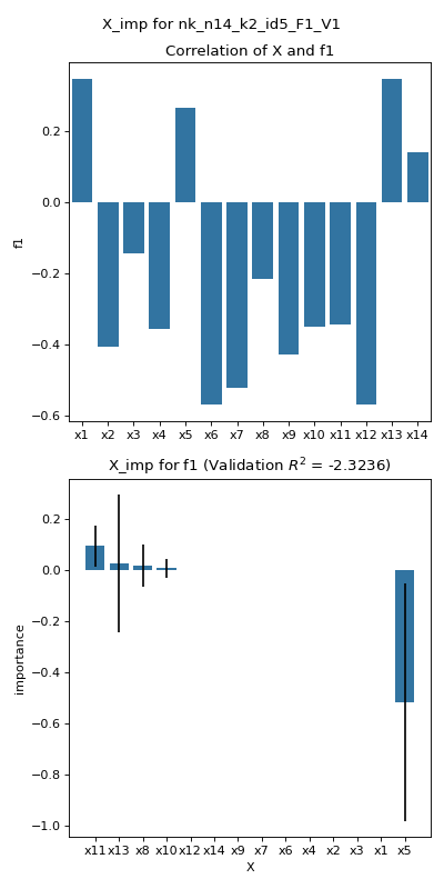

References

[1]

Kalyanmoy Deb. An efficient constraint handling method for genetic algorithms. Computer methods in applied mechanics and engineering, 186(2-4):311–338, 2000.

[2]

José Alexandre F Diniz-Filho, Thannya N Soares, Jacqueline S Lima, Ricardo Dobrovolski, Victor Lemes Landeiro, Mariana Pires de Campos Telles, Thiago F Rangel, and Luis Mauricio Bini. Mantel test in population genetics. Genetics and molecular biology, 36:475–485, 2013.

[3]

Terry Jones, Stephanie Forrest, and others. Fitness distance correlation as a measure of problem difficulty for genetic algorithms. In ICGA, volume 95, 184–192. 1995.

[4]

Monte Lunacek and Darrell Whitley. The dispersion metric and the cma evolution strategy. In Proceedings of the 8th annual conference on Genetic and evolutionary computation, 477–484. 2006.

[5]

Leonardo Vanneschi, Manuel Clergue, Philippe Collard, Marco Tomassini, and Sébastien Vérel. Fitness clouds and problem hardness in genetic programming. In Genetic and Evolutionary Computation Conference, 690–701. Springer, 2004.

[6]

Sébastien Verel, Philippe Collard, and Manuel Clergue. Where are bottlenecks in nk fitness landscapes? In The 2003 Congress on Evolutionary Computation, 2003. CEC'03., volume 1, 273–280. IEEE, 2003.